Introduction
Matrix Action
Perpframes, Aligners and Hangers
Stretchers
Coordinates
Projections
SVD
Matrix Subspaces
Linear Systems, Pseudo-Inverse
Condition Number
Matrix Norm, Rank One
Data Compression
Noise Filtering
Todd Will
UW-La Crosse
Stereo Vision
Heart Model
Best View
Noise Filtering
Noisy Cameras
Filtering
Exercises
In this section you'll see an example where the data in the original matrix is imperfect and the data actually improves when you use a lower rank approximation.
Background: Measuring 3-D motion of the heart in a stereoscopic X-ray set-up
Here is a description of a very recent project byArno Muijtjens, Arie Hasman, Sjef Roos, T. Arts*, R. Reneman**
that uses SVD analysis in biomedical imaging.
The full text can be found at http://www.mi.rulimburg.nl/mi/3dmot.htm
The mechanics of the ventricular wall are investigated as part of the research of the Cardiovascular Research Institute Maastricht (CARIM) of division 5 - Myocardium and Cardiac Activation. The project described here aims at the development of methods for the measurement of ventricular 3-D motion and deformation, using a stereoscopic X-ray stereo set-up and implanted radiopaque markers in combination with video.
Motion and deformation of the left ventricular wall may be quantified by following the motion of markers as a function of time. The 3-D position of the markers can be reconstructed from the two 2-D projections which are obtained in a X-ray stereo set-up. The 3-D trajectories of the markers can be reconstructed when time sequences of frames in two projections are available.
To measure local deformation accurately, large numbers of spherical
markers have to be employed (>10). When reconstructing 3-D trajectories
of many markers, three major problems arise:
-> corresponding markers have to be identified in consecutive frames
(marker tracking), as well as in stereo pairs of frames (stereo correspondence),
-> the accuracy of the marker position measurements has to be increased
by reducing the noise,
-> the parameters describing the unknown geometry of the stereoscopic
X-ray set-up have to be estimated by calibration.
The position of a marker in a frame is represented by a coordinate pair
(x,y).
A chain of (x,y) coordinate pairs represents the track of a marker
in the projection plane. The set of tracks corresponding with M markers
observed in a sequence of T frames is represented by a 2M x T matrix of
marker coordinates as a function
of time.
An efficient method to reduce the noise in marker tracks has been developed by utilizing the coherence of motion in a set of markers. The marker coordinate matrix is approximated by a lower rank matrix which is obtained by truncation of the Singular Value Decomposition (SVD) of the original matrix (SVD-filtering). The method has been evaluated in a computer simulation and in a physiological experiment.
The SVD-filtering method requires a complete set of marker tracks. Often
the tracks are incomplete because of detection failures. Ambiguity with
respect to the identity of detected markers was also occur when tracks
get very close or even cross in the 2-D projection. The SVD- based lower
rank approximation method has been modified to cope with missing position
data.
Stereoscopic Vision
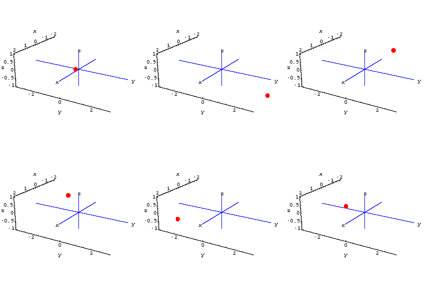
A red fly is buzzing around the room.The location of the fly at time t is
Here's the fly in action:
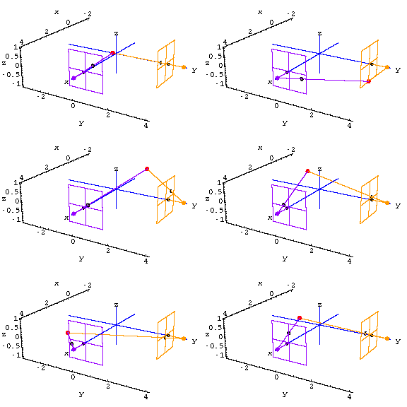
The purple camera is located at the purple dot, {4,0,0}.
The orange camera is located at the orange dot, {0,4,0}.
Both cameras point toward the origin.
When you run a line from the purple camera to the fly (red dot), the line intersects the theoretical screen.
This intersection point tells you where the fly will appear to be on a real screen for the purple camera.
Here the purple grid is located one unit away from the purple camera and is in the plane x=3.
(The location of the theoretical screen depends in part on the lenses
of the camera.)
Here is the 3D view of the fly at time t=10 combined with what each camera records on its own screen:
![[Graphics:noisegr2.gif]](noisegr2.gif)
As seen by the purple camera at time t=10 the fly has approximate screen coordinates {0,0.2}.
As seen by the orange camera at time t=10 the fly has approximate screen
coordinates {0.5,0.25}.
Here's what the two screens look like as the fly buzzes around the room
for times ![]() .
.
Exercises 1-3 below ask you to predict the location of the fly based on its screen coordinates.
Model of the Heart
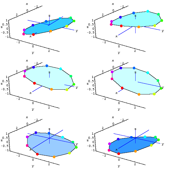
Here's our model of the ventricular wall.The colored dots represent the implanted radiopaque markers.
Best View?
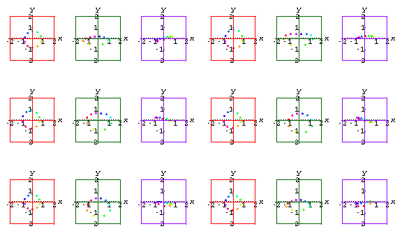
Now let's film the heart with X-ray cameras from three different directions.
Perfect Cameras
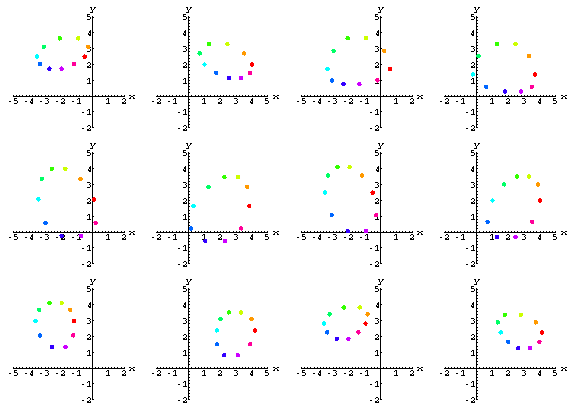
Here are the screen coordinates of the markers as recorded by two cameras.![[Graphics:noisegr5.gif]](noisegr5.gif) .
.The matrix has ten rows, one for each of the markers on the heart.
Each row records the (x,y) screen coordinates of the given marker over
time.
When you perform an SVD on the data in the PerfectCamera matrix you find that the singular values are:
![]()
Not the big drop from the ![]() to
to ![]() .
.
Noisy Cameras
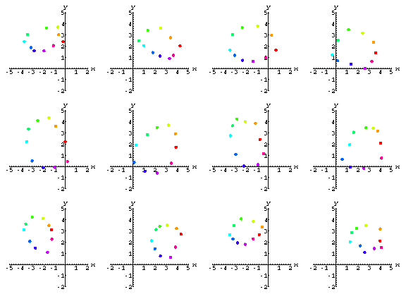
The real world doesn't have perfect cameras.The screen coordinates will inevitably contain noise.
Here's what the data might look like using real world cameras.
![[Graphics:noisegr9.gif]](noisegr9.gif)
The singular values of NoisyCamera matrix are:
![]()
Note that the big drop is gone.
Noise Filtering
Look at the singular values of the two matrices again:PerfectCamera: ![]()
NoisyCamera: ![]()
In the perfect data, the singular values drop off quickly, but in the noisy data, the singular values only gradually get smaller. What causes this?
Evidently, it's the noise in the real camera data that prevents the singular values from dropping off.
Since the noise is what's making the singular values bigger, maybe we
can get rid of the noise by setting these values to zero!
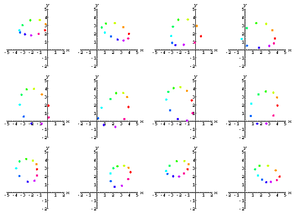
Let FilteredCamera be the rank 5 approximation to the NoisyCamera data.
Here's what the FilteredCamera data look like on each screen.
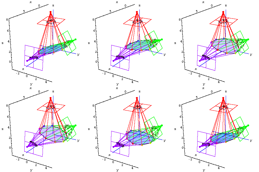
But for proof of success check out the following reconstructions of the heart.
The heart on the left is the reconstruction using the NoisyCamera data.
The heart in the middle is the exact model.
The heart of the right is the reconstruction using the FilteredCamera data.
The reconstruction based on the filtered data on the right looks much better!
The lower rank approximation has removed most of the noise from the
data.
Exercises
1. If the fly is at (2,1,1) what are the purple screen coordinates?Hint: Remember that the purple camera is at {4,0,0} and its theoretical screen is the plane x=3.
To find the purple screen coordinates you'll need to find where the 3D line from the camera to the fly intersects the plane x=3.
2. Suppose at time t=5 you find that the fly has purple screen coordinates
Use this information alone to predict the true location of the fly.
Hints:
-
The line from the purple camera to the fly runs from {4,0,0} through the
point
![[Graphics:noisegr15.gif]](noisegr15.gif) on the theoretical purple screen.
on the theoretical purple screen. - The line from the orange camera to the fly runs from {0,4,0} through the point {3,0,-1} on the theoretical orange screen.
- The fly will be at the intersection of these two lines.
3. Suppose the fly has purple screen coordinates of
Use this information to predict the location of the fly.
Hints:
-
The line from the purple camera to the fly runs from {4,0,0} through the
point
![[Graphics:noisegr18.gif]](noisegr18.gif) on the theoretical purple screen.
on the theoretical purple screen. -
The line from the orange camera to the fly runs from {0,4,0} through the
point
![[Graphics:noisegr19.gif]](noisegr19.gif) on the theoretical orange screen.
on the theoretical orange screen. - Since the screen coordinates are only approximate, these two lines might not intersect. But you can find out where these two lines are closest to each other.
4. Based on the background reading which of the camera angles will be most difficult to use? Why?
5. In our study of the heart, we created a theoretical model of the heart and used this model to create data for our perfect cameras.
When we studied the perfect data generated from our theoretical model we saw a big drop between the 5th and 6th singular values.
This suggested that we use a rank 5 approximation to our NoisyCamera data.
For a real heart, you never get to see perfect data--all you ever have is the data from the noisy cameras.
Speculate on how you might decide on the appropriate rank approximation
for this data.
